This isn’t just another incremental update in simulation tech; it’s a fundamental shift in how we approach design. We’re moving from educated guessing to data-driven evolution. This is one of those advanced CFD techniques that, once you grasp it, makes you wonder how you ever worked without it.
1. Why Traditional Brute-Force Design Iterations are Failing in a Fast-Paced Market
I remember a project early in my career—optimizing a simple HVAC duct bend to reduce pressure drop. We spent three weeks setting up and running over 40 different simulations, tweaking radii and guide vane angles one by one. It was a classic “brute-force” parametric study. We got a decent 8% improvement, but we always had that nagging feeling: was that really the best we could do? Did we miss a non-intuitive shape that would have performed even better?
That’s the core problem. The traditional design loop is slow, expensive, and limited by our own imagination. In a market where time-to-market is everything, spending months on iterative guesswork is a luxury no one can afford anymore. You’re always racing against the clock and computational budget, and often settling for “good enough” instead of truly optimal.
2. What is the Adjoint Solver? An Intuitive Guide for Engineers (Not Mathematicians)
Forget the dense mathematical papers for a second. Think of the Adjoint solver as a kind of ‘performance GPS’ for your design.
A standard CFD solver answers the question: “Given this shape, what is the flow behavior and performance?” (e.g., “What’s the drag on this car body?”).
The Adjoint solver answers a much more powerful question: “To improve my performance objective (like reducing drag), how should my shape change everywhere on its surface?”
It runs a single, clever simulation that produces a “sensitivity map” across your entire geometry. This map literally shows you which areas of your design are most sensitive to change and in which direction (e.g., push this surface in, pull that one out). It’s a roadmap to the perfect design. So, Shape Optimization with the Adjoint Solver isn’t about testing a few ideas; it’s about letting the physics guide you to the best possible idea. 💡
From “What-If” to “What’s Best”: How Adjoint Pinpoints Design Weaknesses
The old way was a series of “what-if” questions. “What if I make the spoiler 5 degrees steeper?” “What if I round this edge more?” You were the one asking all the questions.
The Adjoint method flips this entirely. It tells you what’s best. It highlights the exact regions on your model that are hurting performance. A high-sensitivity spot on the back of a side-view mirror, for instance, is the solver screaming, “Hey! This little area is generating a ton of drag. Fix it!” This shifts your role from a guesser to a strategic decision-maker guided by hard data.
Understanding Sensitivity Maps: Your Visual Guide to a Perfect Shape
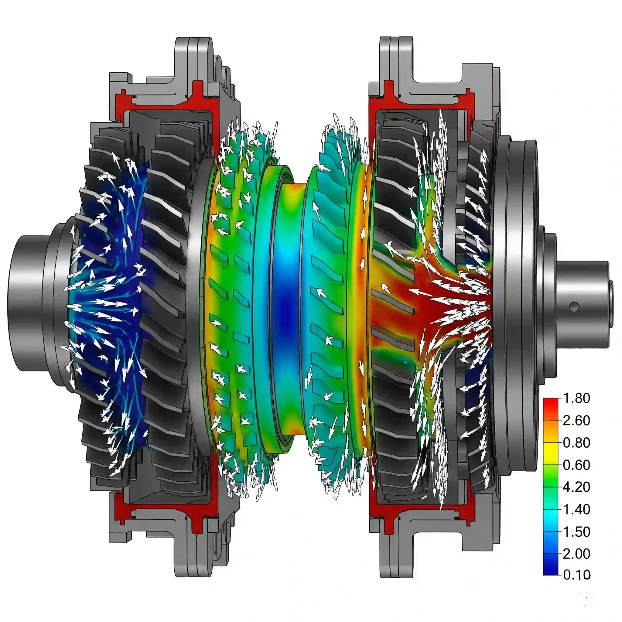
The output of an adjoint simulation is often a colorful contour plot overlaid on your geometry. It’s deceptively simple to read. Typically, red areas indicate surfaces where an outward push (or adding material) will improve your objective (e.g., increase downforce). Blue areas are the opposite; they need to be pushed inward (or have material removed).
It’s an incredibly powerful visual tool. You instantly see the ‘aerodynamic hotspots’ or ‘thermal bottlenecks’ without needing to run dozens of simulations. This becomes especially critical when you’re simulating complex or moving geometries, where manual iteration would be nearly impossible.
3. Adjoint Method vs. Parametric Studies: A Head-to-Head Comparison
I’ve seen projects get completely bogged down in parametric loops, trying to optimize just 5 or 6 variables. The Adjoint method blows that limitation out of the water because it treats the entire surface mesh as thousands of potential variables. The difference is stark.
Here’s a quick cheat sheet based on what we’ve seen on real projects:
| Feature | Parametric “Brute Force” Study | Adjoint Solver Method |
| Design Freedom | Low. Limited to pre-defined parameters you choose. | High. Can discover non-intuitive shapes you’d never imagine. |
| Speed to Insight | Slow. Requires N+1 simulations for N parameters. | Fast. One adjoint run gives sensitivity for the whole surface. |
| Setup Complexity | Initially seems simpler, but becomes complex with many variables. | Higher initial setup effort (defining objective, morphing regions). |
| Computatinal Cost | Very high for comprehensive studies. | Significantly lower for discovering optimal design direction. |
4. The CFDSource 5-Step Workflow for Adjoint-Based Optimization in Ansys & Star-CCM+
Getting a meaningful result from the Adjoint solver isn’t just about clicking a button. It requires a structured, engineering-led process. Over the years, we’ve refined a workflow that avoids common pitfalls and ensures the final design is both optimal and manufacturable. While the specifics can get quite involved, which is why many companies seek out our comprehensive CFD Analysis Services, the core steps are logical.
Here’s a simplified look at how we approach it:
- Step 1: Defining a Clear Objective Function (e.g., Minimize Drag, Maximize Heat Transfer)
This is the most critical step. You have to tell the solver exactly what you want to achieve. “Improve performance” is too vague. Is it minimizing pressure drop across a valve by 10%? Maximizing the uniformity of flow at an outlet? Or perhaps minimizing the peak temperature on a heatsink? A poorly defined objective will send you on a wild goose chase. You also define your constraints here—for example, “don’t change the bolt locations.” - Step 2: Running the Adjoint Solver & Interpreting the Crucial Sensitivity Data
Once the baseline CFD is run, you execute the adjoint solver. The result, as we discussed, is the sensitivity map. The real skill here isn’t just seeing the red and blue spots; it’s interpreting them. Sometimes, a high-sensitivity region is not practical to change due to manufacturing constraints. This is where engineering experience meets the raw data. It’s also where you can start automating parts of the CFD workflow with scripting to streamline how this data is extracted and processed for the next step.
Step 3: Automated Geometry Morphing with Integrated Mesh Deformation
This is where the real magic happens. The software takes that sensitivity map and uses it to physically push and pull the mesh nodes, deforming the geometry towards a better shape. It’s an automated sculptor guided by physics. But you can’t just let it run wild. A poor morphing setup is the fastest way to get junk cells (think skewness > 0.95), which will cause your solver to diverge instantly.
The trick is to define the morphing region intelligently. You need to give it freedom to work, but also constrain it with manufacturing limits. It’s a different kind of meshing challenge compared to, say, using adaptive mesh refinement for grid independence, but the core principle of maintaining a high-quality mesh throughout the process is exactly the same.
Step 4: Validation and Analysis of the Optimized Design
The job isn’t finished once you have a new shape. You have to prove it’s actually better. We always run a final, standard CFD simulation on the new, optimized geometry from scratch. This validates the predicted improvement. Sometimes the adjoint solver predicts a 12% reduction in drag, and the final validation run shows 10%. That’s a huge win, and it’s the number you can confidently take to your design meeting.
For complex validation goals, standard post-processing isn’t always enough. We’ve had projects where the objective was a custom performance index that didn’t exist in the software. In those cases, you often have to extend Fluent’s capabilities with custom functions (UDFs) to measure exactly what the client needs.
5. Real-World Impact: Where CFDSource Leverages Adjoint Solvers for Clients
This isn’t just theoretical. We use this approach to solve tangible, high-stakes problems for our clients.
Case Study Snippet: Reducing Aerodynamic Drag in Automotive Applications by 15%
We worked on an EV project where the side-view mirror was creating a significant amount of aerodynamic noise and drag. The design team had tried three different housings with minimal success. The adjoint solver didn’t suggest a radical new shape. Instead, it pointed to a tiny, almost imperceptible change—a subtle re-sculpting of the underside of the mirror housing. It was a change no human designer would have likely stumbled upon, and it reduced the drag contribution from that single component by over 15%.
Case Study Snippet: Optimizing Internal Flow Channels in Heat Exchangers for Peak Performance
For a client in the electronics cooling industry, the challenge was eliminating hotspots on a new CPU cold plate. The internal micro-channels had recirculation zones where flow was slow and heat transfer was poor. Instead of just making the channels bigger (which would increase the pressure drop), the adjoint solver reshaped the channel inlets and bends. The result was a much more uniform flow distribution, a 20% reduction in peak temperature, all with a negligible impact on the required pumping power.
6. Common Pitfalls and How Our Experts at CFDSource Avoid Them
The path to a great adjoint-optimized design is paved with potential mistakes. One of the classic ones is over-constraining the solver. You tell it to optimize a part but lock down all the important surfaces, essentially tying it’s hands behind its back. You have to give it design freedom.
Another is trusting the first result blindly. Adjoint is a guide, not a dictator. It points you in the right direction, but engineering judgement is still required to interpret the results and decide which changes are practical and manufacturable. A small typo can happen anywhere, even in a report. This is why having an experienced engineer, whether in-house or a consultant like a dedicated CFD freelancer, is so crucial to steer the process.
7. Evolving Your Design Process: The Adjoint Mindset
Ultimately, this is about more than just a new button in your CFD software. It’s a shift in design philosophy. You move from being the sole source of ideas to being the curator of ideas generated by the physics itself. It encourages you to ask better, more open-ended questions.
Instead of asking, “Is design A better than design B?”, you start asking, “What is the best possible design within these constraints?” This approach unlocks a level of performance and innovation that is simply out of reach for traditional iterative methods. Embracing adjoint-driven shape optimization is about forming a partnership between the engineer’s intuition and the raw, unbiased truth of the physics, leading to truly next-generation products.