So you’ve run your simulations. The RANS model converged nicely, your residuals look great, and you have some colorful plots to show for it. But then you get the test data back, and reality doesn’t quite match. Maybe there’s a hot spot the simulation missed, or an unexpected vibration that your steady-state model was blind to.
I’ve been there. In my first few years doing this, about 15 years ago, I was working on a seemingly simple electronics cooling project. My k-epsilon model said the fan placement was perfect. But the prototype kept failing. It turned out a tiny, transient recirculation bubble was forming and starving a critical component of airflow—something my “stable” simulation couldn’t possibly see. That’s the moment you realize standard methods have a ceiling. This guide is about what lies beyond that ceiling, covering the advanced CFD techniques that tackle the truly messy, complex problems we face in modern engineering.
Beyond the Basics: When Standard CFD Simulations Reach Their Limits
The standard toolbox—think RANS models like k-epsilon and k-omega—is fantastic for a huge range of problems. They are the workhorses of the industry. But they are based on time-averaging assumptions that start to fall apart when the physics gets complicated.
You know you need to level up when your project involves:
- Massive Separation & Transient Vortices: Think flow over a bluff body, like a truck, or the unsteady wake behind a turbine blade.
- Strong Multiphysics Coupling: When the fluid flow deforms the solid structure, or the thermal state of a solid fundamentally changes the fluid behavior.
- High-Fidelity Acoustics: Predicting the noise generated by airflow, not just the flow itself. ✈️
- Complex Phase Change: Situations like cavitation in a pump or boiling inside a heat pipe where performance is dictated by bubble dynamics.
Here’s a quick cheat sheet on where the lines are drawn:
| The Challenge | Standard RANS Approach | Advanced CFD Solution |
| Predicting unsteady wake turbulence | Gives a time-averaged, “blurry” picture. | LES/DES to resolve the actual turbulent eddies. |
| Structure deforms due to fluid load | Requires manual iteration or simplified coupling. | Fully-coupled Two-Way FSI simulations. |
| Heat transfer through solid & fluid | Run separate models or use simplified BCs. | Conjugate Heat Transfer (CHT) for a holistic view. |
| Simulating droplet spray | Often uses simplified Lagrangian particle tracking. | Volume of Fluid (VOF) to capture the interface shape. |
Category 1: Tackling Complex Physics with Advanced Modeling
Alright, let’s get into the good stuff. The first major leap in advanced CFD is moving beyond simplified physics. It’s about letting the simulation capture more of the real-world interactions that actually govern a system’s performance. This isn’t just about getting a more accurate number; it’s about discovering phenomena you didn’t even know existed.
Multiphysics Simulations: When One Physics Isn’t Enough
Things in the real world don’t happen in a vacuum. A winglet deflects because of air pressure. An engine block gets hot because of the combustion and coolant flow. Multiphysics is about simulating these interactions directly, instead of making educated guesses. It’s where CFD stops being just about fluids and starts being about systems.
For a detailed walkthrough on coupling fluid dynamics with structural mechanics, especially when the solid’s deformation affects the flow, see our guide on A Practical Guide to Two-Way Fluid-Structure Interaction (FSI) Simulations. And for thermal applications, where the heat flow between a solid and fluid is critical, mastering the synergy between them is essential. We break that down in Mastering Conjugate Heat Transfer (CHT) for Comprehensive Thermal Management. It’s a game-changer for electronics cooling and engine design.
Capturing Extreme Flow Regimes: From Sound Waves to Shock Waves
When you push speeds up, the physics changes dramatically. Standard incompressible solvers just can’t handle it. This is the domain of high-speed aerodynamics and aeroacoustics, where things get really interesting (and computationally expensive 😅). It’s not just about drag and lift anymore; it’s about shockwave locations, sonic booms, and noise generation.
You can’t use a standard CFD solver to find out why a landing gear is so noisy. For that, you need a specialized approach, which we cover in our introduction to Aeroacoustics (CAA) with CFD. And when you’re dealing with flows exceeding the speed of sound, the entire simulation strategy has to be different. We dive into those unique challenges and best practices for Simulating Supersonic and Hypersonic Flows.
Advanced Material & Chemical Modeling
Sometimes the fluid itself is the biggest challenge. Water and air are simple, but what about polymer melts, blood, or drilling mud? Their viscosity changes with stress, and you can’t just plug in a constant value. Modeling these materials correctly is the key to designing everything from more efficient food processing equipment to better biomedical devices. We cover the simulation of these complex materials in our guide to Modeling Non-Newtonian Fluids in CFD.
In high-temperature systems like furnaces or combustion chambers, another factor dominates: thermal radiation. It’s often the primary mode of heat transfer, and picking the wrong model can throw your temperature predictions off by hundreds of degrees. We’ve seen projects where a simple model choice completely changed the predicted outcome of it’s performance. That’s why we wrote a guide on Choosing the Right Radiation Model in CFD (DO, P1, S2S) to help you navigate those options.
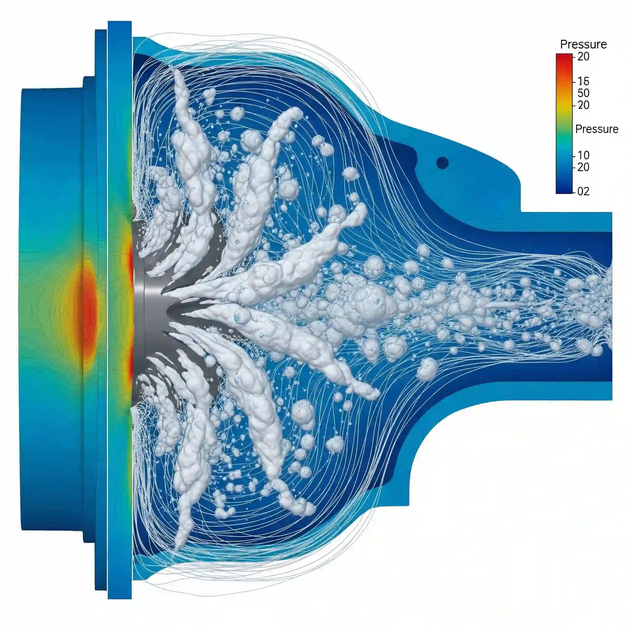
Phase Change and Multiphase Flow Phenomena
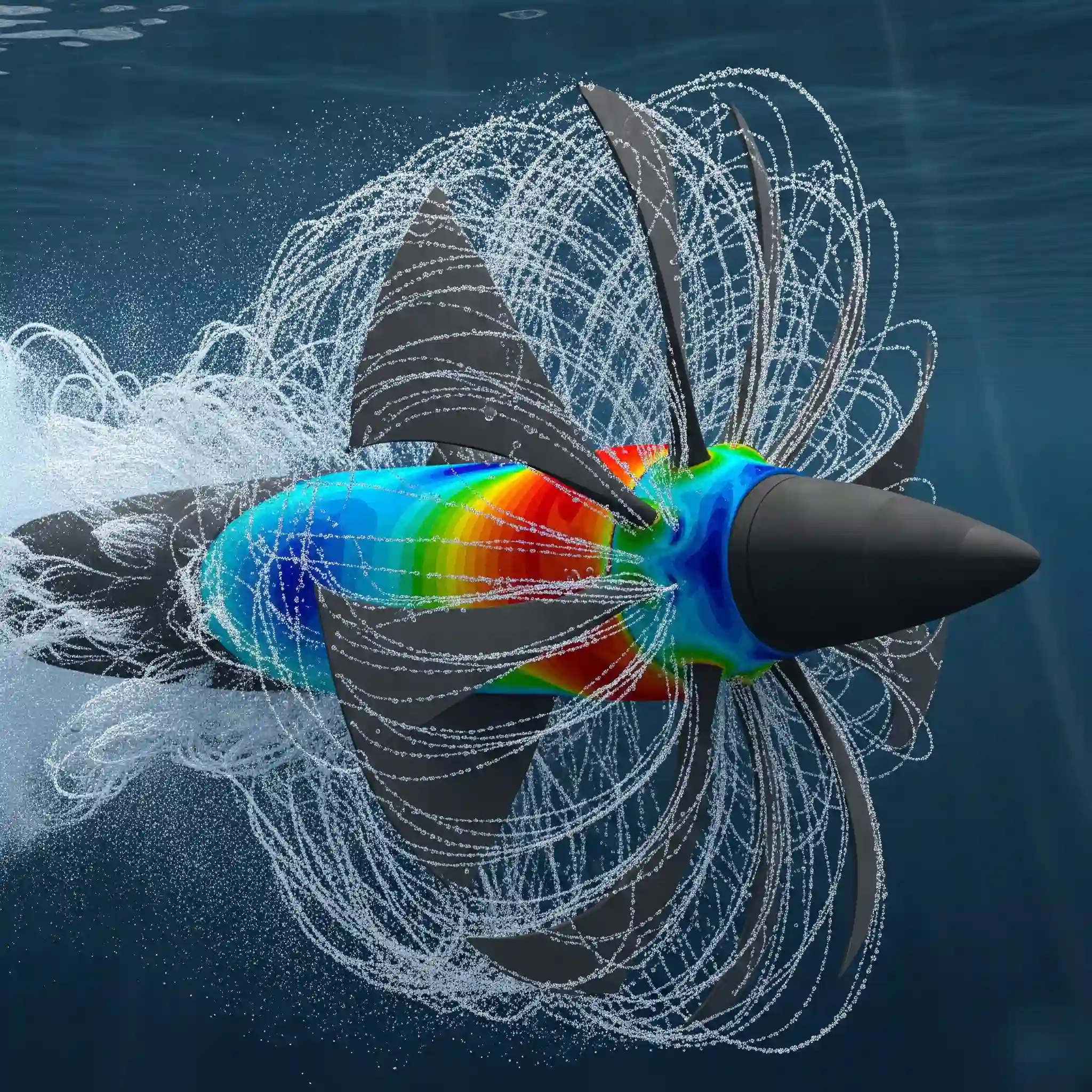
When you have more than one phase—liquid and gas, for instance—or when one phase is turning into another, you’re in the realm of multiphase flow. This can be as subtle as predicting humidity condensation or as violent as the destructive collapse of cavitation bubbles on a ship’s propeller.
Accurately capturing the interface and the physics of phase change is critical for these applications. A small error in predicting the vapor pressure can mean the difference between a functional pump and one that destroys itself in weeks. You can discover how to use modern CFD simulation techniques to Predict and Mitigating Cavitation in Pumps and Hydrofoils using CFD, a problem that costs the marine and turbomachinery industries millions every year.
Category 2: Advanced Methodologies & Solver Technologies
Okay, so we’ve talked about modeling more complex physics. But how do the solvers actually handle this? This next part is about the engine under the hood—the numerical methods and technologies that make solving these tough problems possible. This isn’t just academic; choosing the right methodology can be the difference between a simulation that converges in a day and one that runs for a month before crashing.
The Turbulence Dilemma: When to Move Beyond RANS
This is probably the most common crossroads in CFD. RANS is fast, robust, and gives you a decent, time-averaged answer. But that “time-averaged” part is the catch. It smears out all the beautiful, chaotic, and often critical, transient details of turbulence. It gives you the climate, when what you really need is the weather.
I saw this firsthand on an automotive project, looking at the flow around a side mirror. The RANS model showed a smooth, attached wake. The wind tunnel test, however, showed a pulsating, oscillating wake that was creating a really annoying whistling noise. The problem wasn’t the RANS model’s accuracy; it was it’s fundamental inability to capture that unsteady vortex shedding. Moving to a DES model was like putting on glasses for the first time. Suddenly, we could see the eddies peeling off the mirror. If you’re facing a similar situation, our guide on When to Move from RANS to Large Eddy Simulation (LES/DES) breaks down the decision process.
A Comparative Guide to Multiphase Simulation Models
When you have two or more fluids that don’t mix, like air and water or oil and gas, you need a way to track where one ends and the other begins. The two big players here are Volume of Fluid (VOF) and Eulerian-Eulerian. They approach the problem completely differently.
Think of VOF as a high-definition camera focused on the interface. It’s perfect for things like sloshing in a fuel tank or simulating the shape of a breaking wave. It’s precise, but can be computationally heavy. The Eulerian model, on the other hand, treats the phases as two intermingled “clouds” that occupy the same space. It’s much more efficient for things like bubbly flows in a reactor or fluidized beds where you care more about the volume fraction than the exact shape of every single bubble. We’ve got a full breakdown comparing them side-by-side in our guide: Volume of Fluid (VOF) vs. Eulerian-Eulerian: A Comparative Guide for Multiphase Simulations.
Unlocking Reactive Flows: Advanced Combustion Modeling
Combustion is just incredibly complex. It’s a mix of turbulent flow, intense heat transfer, and dozens of chemical reactions happening in microseconds. Simple models like the Eddy Dissipation Model (EDM) basically assume that the chemistry happens instantly the moment fuel and oxidizer meet. This is fine for predicting the main flame shape, but it’s totally useless for predicting pollutants like NOx or soot, which depend on the finite-rate chemistry.
This is where flamelet models come in. They pre-calculate the complex chemistry in a separate, one-dimensional space and then map it back into your 3D flow field. It’s a brilliantly efficient way to include detailed chemical kinetics without paying the insane computational price of solving for every species transport equation. For anyone working with engines or burners, understanding these advanced CFD techniques is non-negotiable. We get into the nitty-gritty of it in Advanced Combustion Modeling: From Eddy Dissipation to Flamelet Models.
The Pinnacle of Design: Shape Optimization with the Adjoint Solver
This one still feels a bit like magic, even after all these years. For decades, design optimization was a manual loop: the engineer proposes a design change, the CFD analyst runs a simulation, they analyze the results, and the engineer proposes another change. It’s slow and relies heavily on intuition.
The Adjoint solver flips that script entirely. 🔄 Instead of you telling the solver what to change, the solver tells you. It calculates the “sensitivity” of your objective (say, drag) to the shape of every single point on the surface. It essentially creates a map showing you exactly where to push or pull the surface to get the biggest improvement. It’s how you go from a good design to a truly optimal one, automatically. Learn more about this powerful method in our article on Shape Optimization with the Adjoint Solver: The Future of Automated CFD Design.
Category 3: The Modern CFD Workflow: Efficiency, Automation & Power
Having powerful solvers is one thing. Being able to use them efficiently is another. The modern workflow isn’t about clicking buttons for one simulation. It’s about building repeatable, automated processes that let you explore the design space, handle insane geometric complexity, and get the most out of your hardware. This is where the real engineering productivity gains are made.
Mastering the Mesh: Techniques for Complex Geometries and High Accuracy
“Garbage in, garbage out” was practically invented for CFD meshing. A bad mesh will give you a bad result, period. Two techniques have fundamentally changed how we handle complex meshing challenges: Overset Mesh and Adaptive Mesh Refinement (AMR).
Overset (or Chimera) mesh is a lifesaver for problems with large, complex relative motion. Think of a missile launching from a plane. Instead of trying to create a single, deforming mesh that will inevitably get tangled and break, you mesh the missile and the plane separately and just let the missile’s mesh move through the background mesh of the air. It’s so much more robust. Check out our “how-to” on Simulating Complex Moving Geometries with Overset Mesh.
AMR, on the other hand, is about being smart with your cells. Why use a super-fine mesh everywhere when you only need high resolution around the shockwave or in the flame front? AMR automatically refines the mesh in high-gradient areas and coarsens it where nothing is happening. It’s the key to Achieving Grid Independence Efficiently with Adaptive Mesh Refinement (AMR) without needing a supercomputer for every run.
Automation and Customization: Beyond the GUI
If you’re still doing everything by clicking through menus in the software’s graphical user interface (GUI), you’re leaving a massive amount of efficiency on the table. The real power comes when you go “under the hood” and start scripting. It feels intimidating at first, but once you start, you’ll never go back.
For example, I once had to run 50 variations of an impeller design, each with a slightly different blade angle. Doing that manually would have been a week of mind-numbing, error-prone clicking. Instead, I spent a day writing a simple Python script. The script built the geometry, meshed it, ran the simulation, and even extracted the key performance data into a spreadsheet. The whole thing then ran by itself over the weekend. That’s the power of Automating Your CFD Workflow with Python Scripting in Ansys Workbench.
Sometimes the built-in physics models aren’t quite right. Maybe you have a proprietary material property or a unique source term. This is where User-Defined Functions (UDFs) come in. They are snippets of C code that hook directly into the solver, letting you define your own rules for the simulation. It’s the ultimate customization tool, and we cover the basics in Extending Ansys Fluent’s Capabilities with Custom User-Defined Functions (UDFs).
Handling the Scale: Supercomputing and Big Data
When you start running LES or DES simulations on complex geometries, the file sizes get ridiculous. We’re not talking megabytes or even gigabytes anymore; we’re talking terabytes. A single transient simulation can easily generate 10-20 TB of data. Just opening one of these result files can crash a standard workstation.
This is where High-Performance Computing (HPC) becomes a necessity, not a luxury. But using an HPC cluster isn’t just about having more cores. It’s about understanding how to partition your mesh effectively, how to manage the massive I/O load, and how to minimize communication latency between nodes. It’s a skill in itself. We share some hard-won lessons in our Best Practices for High-Performance Computing (HPC) in Large-Scale CFD Simulations.
And once you have all that data, what do you do with it? You can’t just scroll through thousands of timesteps looking for interesting events. You need strategies for data reduction and targeted post-processing. We discuss techniques like creating temporal statistics on-the-fly and using data extract scripts in Strategies for Handling and Post-Processing Terabyte-Scale CFD Datasets.
Category 4: The Future of Simulation: AI, Reliability, and Digital Integration
So, what’s next? Where is all of this heading? The field is moving incredibly fast, and the focus is shifting from just generating predictions to generating reliable, fast, and integrated predictions that can drive real-time decisions. This is the bleeding edge, and it’s incredibly exciting.
The AI Revolution: Physics-Informed Neural Networks (PINNs)
This one is a real paradigm shift. For decades, we’ve relied on traditional numerical methods (FVM, FEM) to solve the governing equations of fluid dynamics. Now, AI is offering a completely new approach. Physics-Informed Neural Networks (PINNs) are a type of machine learning model that learns to solve these equations.
The crazy part is they don’t need a mesh. They learn the underlying continuous solution directly. While still an emerging field, the potential is staggering: imagine getting near-instantaneous CFD results for design iterations or using them as real-time surrogate models. It’s a fascinating topic, and we scratch the surface in The Rise of Physics-Informed Neural Networks (PINNs) and AI in CFD. It’s going to change everything in the next decade.
From Prediction to Certainty: Quantifying Uncertainty in CFD
Every engineer has been asked this question: “Okay, the simulation says 450 Kelvin… but how much do you trust that number?” For a long time, the answer was a shrug and “it’s a good estimate.” That’s not good enough anymore, especially in high-stakes industries like aerospace or nuclear.
Uncertainty Quantification (UQ) is the formal process of putting error bars on your CFD results. It accounts for uncertainties in your inputs—things like manufacturing tolerances, material properties, or boundary conditions—and propagates them through the simulation to see how much they affect the final output. It’s the difference between saying “the lift is 1000 N” and saying “we are 95% confident the lift is between 980 N and 1020 N.” Learn more in our Introduction to Uncertainty Quantification (UQ) for More Reliable CFD Predictions.
The Ultimate Application: Building a CFD-Based Digital Twin
This is where everything we’ve talked about comes together. A digital twin is a virtual replica of a physical asset, updated in real-time with sensor data from its real-world counterpart. It’s not just one simulation; it’s a living model that evolves with the actual product. ⚙️
CFD is a cornerstone of this concept. You can use high-fidelity models to build the initial twin, and then use AI/ML surrogate models (like the PINNs we mentioned) to run fast enough for real-time operation. Imagine a wind turbine’s digital twin that uses live wind data to adjust its blade pitch for maximum efficiency and minimum structural load, all based on a constantly running CFD model. It’s the ultimate goal of predictive engineering. We outline the roadmap in Building a CFD-Based Digital Twin: From Concept to Real-Time Operation.
The CFDSource Framework: A Pragmatic Approach to Selecting the Right Technique
With so many advanced methods, how do you choose the right one for your job without wasting time or computational resources? It comes down to asking the right questions. Over the years, we’ve developed a sort of mental checklist to guide this decision. It’s less about a rigid flowchart and more about a pragmatic assessment of what you’re really trying to achieve.
Balancing Accuracy vs. Computational Cost: A CEO’s and an Engineer’s Perspective
This is the conversation that happens on every single project. The engineer wants to run a high-fidelity LES on a 100-million-cell mesh to capture every last wisp of turbulence. The manager (or CEO) sees the quote for the cloud computing hours and asks, “Can’t we just get a ‘good enough’ answer with RANS?”
Both perspectives are valid. The key is to connect the required physical accuracy to a tangible business outcome. For example, on a project optimizing an F1 car’s front wing, a 0.5% drag reduction is worth millions. Here, the enormous cost of a DES or LES simulation is easily justified. For designing a simple ventilation system in a garage, a RANS model that’s within 10-15% of reality is perfectly fine. The extra cost of LES buys you nothing of value.
It’s not about always using the most advanced tool; it’s about using the sharpest tool for the specific job. I remember a client who insisted on a full LES simulation for a simple heat exchanger. The simulation ran for three weeks. We could have gotten them an answer that was just as useful for their design decision in about four hours with a well-calibrated RANS model. It was a perfect example of computational overkill.
Common Pitfalls in Advanced Simulations (And How Our Experts at CFDSource Avoid Them)
Running advanced simulations is a bit like navigating a minefield. The potential for things to go wrong increases exponentially compared to standard CFD. These aren’t textbook problems; they are messy, and the solvers can be finicky.
Here are a few “scars” from our own projects:
- The FSI Run That Never Converged: In a Fluid-Structure Interaction simulation of a valve, the fluid forces were causing the mesh on the solid side to deform so badly that it inverted (negative volume cells). The run would crash every time. The fix wasn’t in the CFD solver, but in the structural mesh settings, by adding stiffness to prevent the elements from collapsing. It’s a classic multiphysics problem where the issue is at the interface of the disciplines.
- The “Quiet” LES: We once ran a huge LES simulation to predict aeroacoustic noise, but the results showed almost no pressure fluctuations. We spent days debugging the solver settings, only to realize the inlet boundary condition was too clean—it was feeding perfectly laminar flow into the domain. We had to add synthetic turbulence at the inlet to “trip” the flow and generate the realistic eddies we needed. A simple oversight that almost invalidated a week of computation.
- Forgetting about y+: This one’s a classic. An engineer will set up a beautiful DES simulation, but use a standard wall function mesh designed for RANS. The entire simulation becomes garbage because the solver isn’t resolving the near-wall region correctly. Advanced CFD modern techniques demand advanced meshing practices.
Case Study: Solving a Complex Aeroacoustics Challenge for an Automotive Client
We worked with an automotive tier-1 supplier who was developing a new HVAC blower. The prototype was efficient, but it produced an annoying high-pitched “whine” at certain speeds. Their standard RANS simulations couldn’t predict this at all; the flow fields looked perfectly smooth.
They came to us to figure out the noise source. We couldn’t just jump to a full-blown CAA simulation; it would have been too expensive. Instead, we used a hybrid approach. First, we ran a transient DES simulation to accurately capture the turbulent eddies spinning off the tips of the blower blades. This gave us the unsteady pressure sources.
Then, we used the Ffowcs Williams-Hawkings (FW-H) acoustic analogy to project the noise from these sources to a “microphone” location in the far-field. The simulation data clearly showed a tonal noise peak at exactly the frequency the prototype was producing. 🎶 We identified the source as a periodic vortex shedding phenomenon. Using this insight, we suggested a small change to the blade trailing edge geometry. The follow-up simulation showed the tonal peak was gone, and so was the whine in the next prototype.
Conclusion: Advanced CFD Is Not Just a Tool, It’s a Competitive Advantage
As you can see, this stuff goes way beyond just making pretty pictures. When you move past the basics, you’re no longer just verifying designs; you’re actively discovering new physics that can lead to breakthrough innovations. You’re finding that 0.5% efficiency gain, eliminating that unexpected vibration, or creating a product that is significantly quieter than your competitor’s.
It’s not easy. It requires a deep understanding of the underlying physics, the numerical methods, and frankly, a lot of experience with how these simulations can fail. But the payoff is enormous. It’s how you stop being reactive and start being predictive in your engineering design process.
Ready to Tackle Your Toughest Engineering Challenge? Partner with CFDSource.
If you’ve read this far, you’re likely facing a problem where the standard approach isn’t cutting it. Maybe you’re pushing the boundaries of performance, wrestling with a complex multiphysics interaction, or trying to solve a failure that no one can explain.
That’s our sweet spot. At CFDSource, we specialize in applying these advanced techniques to solve real-world industrial problems. We’re not just running software; we’re a team of experienced engineers who understand the connection between the simulation and the physical product. If you have a project that could benefit from this level of analysis, take a look at our case studies to see the kind of problems we solve.