Aeroacoustics (CAA) with CFD: A Practical Engineer’s Guide from Noise Source to Receiver

Why Noise Isn’t Just Annoying—It’s a Critical Engineering Problem

Let’s be honest. For years, many engineers treated noise as an afterthought. A problem for the testing phase. But that mindset is a fast track to expensive redesigns. After spending over a decade in this field, I’ve seen projects get derailed late in the game because a fan blade was “too loud” or a car’s side mirror created an unbearable whistle at highway speeds. This isn’t just about comfort; it’s about passing strict environmental regulations and building products people actually want to use.

Understanding and predicting this noise before you build anything is a huge advantage. It’s a specialized domain that sits right at the intersection of fluid dynamics and acoustics, and it’s a key part of what we explore in [our deep dive into Advanced CFD techniques]. This is where Computational Aeroacoustics, or CAA, comes into play.

The Fundamentals: What is Computational Aeroacoustics (CAA)?

So, what is CAA? Forget the dense academic papers for a second. Think of it as a two-part story.

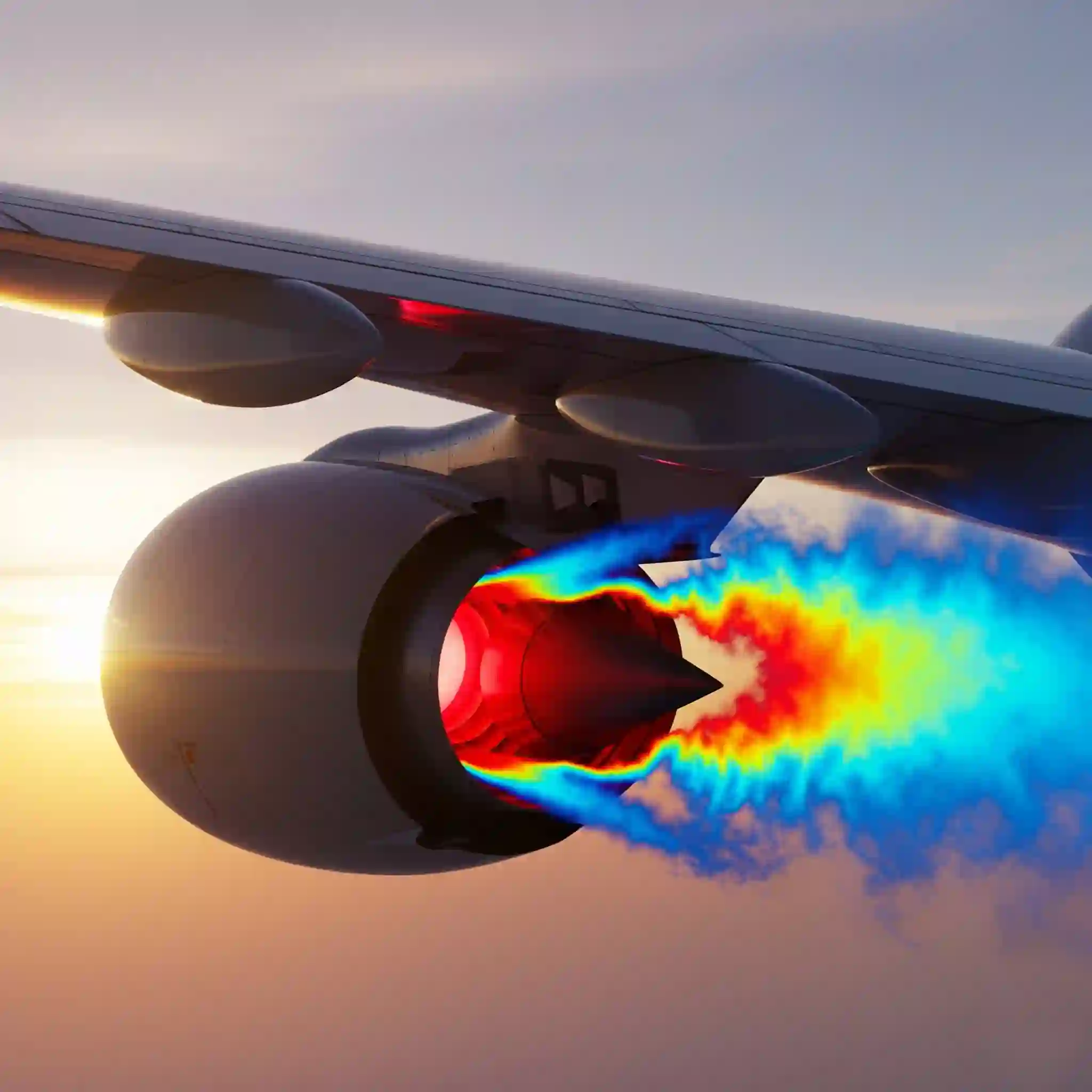
First, we use CFD to simulate the turbulent, messy fluid flow that creates the noise. Imagine the chaotic air tumbling off an airplane wing or the unsteady vortices shedding from a rotating fan. This is the source of the sound. Second, we take the pressure fluctuations from that simulation and calculate how they travel, or propagate, through the air as sound waves to a listener’s ear (the receiver). It’s a powerful hybrid approach that gives us the full picture.

The Core Workflow: How CFDSource Traces Sound from a Turbulent Flow to a Listener

We don’t just throw a model at the wall and see what sticks. There’s a methodology. It always starts with identifying the noise-generating mechanisms. Is it the turbulence itself? Or is it a surface vibrating due to fluid forces, a problem that often requires a [detailed two-way FSI simulation]? Once we know the “what,” we move to the “how.” This involves a very specific type of CFD simulation to capture the source, followed by an acoustic solver to handle the propagation. It’s a delicate process, and getting one part wrong invalidates everything that follows.

Step 1: Capturing the Source – The Unsteady CFD Simulation

This is the most critical and computationally expensive part. You can’t predict sound from a steady-state (RANS) simulation. Sound is, by its very nature, an unsteady phenomenon—a fluctuation. To capture it, you need a simulation that resolves these fluctuations in both space and time.

Why Standard RANS Models Fail for Noise Prediction (And Why We Use LES/DES)

I learned this the hard way early in my career on an HVAC system project. We used a standard k-epsilon model, and the results showed… nothing. No useful acoustic data at all. That’s because RANS models are designed to average out the turbulence, effectively smoothing away the very pressure pulses that create sound. 🤦‍♂️

To actually capture noise sources, you need more advanced turbulence models like Large Eddy Simulation (LES) or Detached Eddy Simulation (DES). These models resolve the large, energy-containing eddies directly and model the smaller ones. This unsteady approach is the foundation for any serious introduction to Aeroacoustics (CAA) with CFD. It’s more demanding, but it’s the only way to get data that reflects reality.

Critical Meshing Strategies: Resolving the Eddies that Generate Sound

Your mesh for a CAA analysis is fundamentally different. It needs to be fine enough not just to capture the boundary layer, but to resolve the acoustic wavelengths of interest. A common rule of thumb is to have at least 10-15 high-quality cells per wavelength for the highest frequency you care about. If your mesh is too coarse, the numerical dissipation will simply kill the acoustic waves before they even form. This is especially challenging in problems with shockwaves, similar to the meshing demands for [simulating supersonic and hypersonic flows]. It’s a balancing act between accuracy and computational cost.

Step 2: Propagating the Sound – Choosing the Right Acoustic Analogy

Running a single, massive simulation that captures both the fluid flow and the sound propagation all the way to the listener is often impossible due to the insane computational cost. The scales are just too different. So, we use a cleverer, more efficient method: acoustic analogies. We run the high-fidelity CFD in a small region around the noise source and then use a mathematical formula to project that sound out into the far-field.

Lighthill’s Analogy: Understanding the Basics of Flow-Induced Noise

Lighthill’s analogy is the granddaddy of them all. It brilliantly reframes the Navier-Stokes equations into a wave equation with a source term. In simple terms, it mathematically proves that unsteady turbulence acts just like a collection of tiny loudspeakers (quadrupoles) broadcasting sound. It provides the theoretical backbone for everything else we do in CAA.

The Ffowcs Williams-Hawkings (FW-H) Model: The Industry Standard for Far-Field Noise

While Lighthill’s is the theory, the FW-H model is the workhorse we use in practice with software like Ansys Fluent or Star-CCM+. It takes the pressure and velocity data from a permeable surface you draw around the noise source in your CFD simulation and uses it to calculate the sound at any specific receiver point, no matter how far away.

It’s an incredibly powerful and efficient method. However, implementing it correctly requires a deep understanding of the physics and the software’s settings. It’s a complex process, which is why many companies find it more effective to partner with specialized [CFD analysis services] rather than trying to develop this niche expertise in-house. This ensures the setup is correct and the results are trustworthy. The whole process is about turning complex fluid data into a simple, actionable result, like a decibel level at the driver’s ear. 🚗

Putting Theory into Practice: A CFDSource Case Study on Automotive Side Mirror Noise

This all sounds great in theory, but what does it look like in a real project? A few years back, an automotive client came to us with a frustrating problem. Their new SUV model had a persistent, high-pitched whistle coming from the side mirrors at speeds above 70 mph. It was driving test drivers crazy and was a potential deal-breaker for production.

Instead of guessing, we built a high-fidelity DES simulation focused on the air flowing around the mirror housing. The CFD results quickly identified the culprit: a sharp edge on the underside of the mirror was causing a very stable, periodic vortex shedding—a perfect recipe for tonal noise. We used the FW-H model to project this noise to the driver’s ear location. The simulation predicted a sharp peak in the noise spectrum right around 2500 Hz, which matched their experimental data almost perfectly.

The best part? The fix was simple. Based on the flow patterns, we recommended a subtle rounding of that specific edge—a change of less than 3mm. We re-ran the simulation with the new geometry, and the tonal peak was gone, replaced by a much lower-level broadband noise. A small design tweak, guided by simulation, saved them from a costly tooling change down the line. That’s the power of this approach.

Common Pitfalls in CAA Simulations and How to Avoid Them

Getting into aeroacoustics isn’t exactly a walk in the park. There are a few classic traps that everyone falls into at first. Knowing them ahead of time can save you weeks of wasted computation and headaches.

The Challenge of High Computational Cost: Our Approach to Efficient Simulation

Let’s be blunt: these simulations are hungry. 🐲 They demand massive meshes and tiny time steps, which means they can run for days or even weeks on a high-performance computing (HPC) cluster. One common mistake is trying to use a super-fine mesh everywhere. It’s just not practical.

Our approach is to be smart about where we spend our computational budget. We use hybrid meshes—a very fine, high-quality LES-level mesh in the critical noise-generating regions, and a more efficient RANS-level mesh further away. This gives us the detail where it matters without burning CPU hours unnecessarily. It’s a trade-off, always, but one you learn to make with experience.

Post-Processing Hell: How to Extract Meaningful Acoustic Data (like SPL Maps)

So your simulation finally finished, and you have 2 Terabytes of transient data. Now what? 🤯 This is where many projects stall. The raw CFD output isn’t the answer; you have to process it to find the acoustic insights. You need to convert raw pressure data into things that engineers and managers actually understand.

This means running FFTs (Fast Fourier Transforms) on pressure signals to get frequency spectrums, plotting Sound Pressure Level (SPL) contours on a 3D surface, and creating directivity plots to see in which direction the sound is loudest. It’s an entire discipline in itself, and without the right scripts and tools, you can easily get lost in the data.

Beyond the Simulation: How We Validate Our CAA Results Against Experimental Data

A simulation is only a model of reality. If you can’t trust its output, it’s useless. That’s why we always insist on validating our results whenever possible. This means comparing our simulated SPL values and frequency spectra against real-world measurements from an anechoic chamber or against data from published academic papers.

We don’t just look for a match in the peak decibel level. We look for a match in the shape of the acoustic signature. Does our simulation capture the right tonal peaks? Is the broadband noise level in the correct range? This level of comparison builds confidence and ensures that the design decisions we make are based on sound—pun intended—data. It’s a critical step that separates predictive engineering from just making pretty pictures.

Is CAA the Right Solution for Your Product? A Quick Checklist

Wondering if this approach is a fit for your specific challenge? Here’s a quick mental checklist:

• Is the primary noise source related to turbulent or unsteady fluid flow? (e.g., HVAC fans, aircraft landing gear, wind turbines). If yes, CAA is likely a good fit.
• Is the noise caused by a different physical phenomenon? For example, the noise from collapsing bubbles is a unique acoustic problem often tied to [predicting cavitation in pumps and hydrofoils]. While CFD is used, the modeling approach is different.
• Are you looking to predict noise at a specific location or in a specific direction? The FW-H method is perfect for this.
• Is your goal not just to measure noise, but to actively reduce it through design changes? This is where simulation truly shines, allowing for rapid virtual prototyping.

Partner with CFDSource: From Noise Analysis to Design Optimization

Ultimately, running a successful aeroacoustic simulation is more than just software skills. It’s about understanding the underlying physics and knowing how to translate complex data into actionable design improvements. We don’t just hand over a report full of charts; we partner with your team to interpret the results and find practical solutions.

Among the many [CFD analysis companies], our focus is on becoming an extension of your R&D team. We provide the specialized expertise to solve your toughest noise problems, letting you focus on what you do best. If you’re tired of chasing noise issues in the testing phase, it might be time to explore how a well-executed analysis from noise source to receiver with CFD can change your design process for the better.