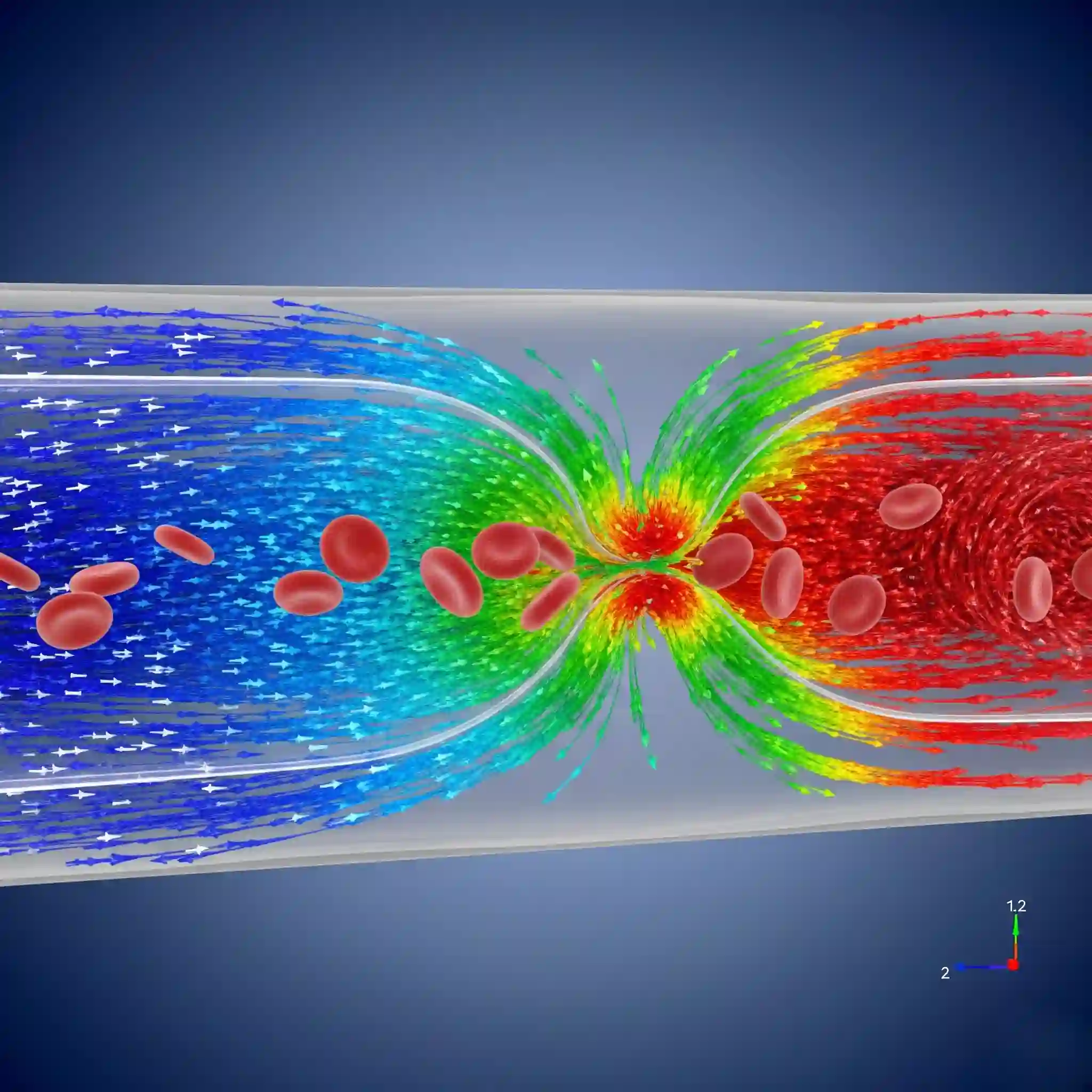
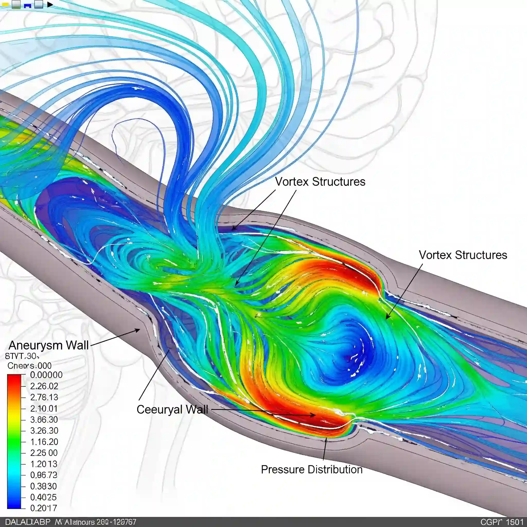
So, you’re trying to simulate something that isn’t water or air. Ketchup, drilling mud, melted plastic, maybe even blood. Suddenly, all the standard rules seem to break, and your simulation either diverges or gives you results that just feel… wrong. You’re in the right place. This isn’t just another textbook overview; it’s a field guide based on real-world projects.
This topic is a key part of our larger series on Advanced CFD Simulation Techniques, where we break down the toughest challenges in the field. But for now, let’s get our hands dirty with fluids that refuse to behave. We’re going to cover the essential models and practical steps for modeling non-newtonian fluids in CFD, so you can get results you can actually trust.

Why Your Standard CFD Approach Fails: The Critical Difference Between Newtonian and Non-Newtonian Fluids
Forget the complex equations for a second. The core difference is simple: a Newtonian fluid (like water) has a constant viscosity no matter how much you stir it. A non-Newtonian fluid doesn’t. Its viscosity changes with the forces applied to it (the shear rate).
Think about a bottle of ketchup. It’s thick and stubborn in the bottle (high viscosity). But when you shake it hard or squeeze it (high shear rate), it suddenly flows easily (low viscosity). That changing behavior is everything. If you define ketchup in your CFD software with a single viscosity value, your simulation of squeezing the bottle will be completely wrong. It’s this shear-dependent viscosity that we need to capture.
Choosing Your Weapon: A Practical Guide to Non-Newtonian Rheological Models
There’s a whole toolbox of mathematical models to describe this behavior, and picking the right one is half the battle. You don’t need to know all of them, but you absolutely must know the main players and where they shine. It’s not about which model is “best,” but which model is best for your specific material and flow conditions.

The Workhorse Models: Power Law for Polymers and Shear-Thinning Fluids
The Power Law model is probably the most famous. It’s simple, robust, and does a fantastic job for many materials that are “shear-thinning” (viscosity decreases as shear increases), like polymer melts or paint.
It uses two main parameters: the consistency index (k) and the flow behavior index (n). If n < 1, the fluid is shear-thinning. If n > 1, it’s shear-thickening (like a cornstarch and water mix). Its a great starting point, but be careful: it isn’t accurate at very low or very high shear rates, where many fluids tend to plateau. For some processes, that limitation can be a deal-breaker.
For Yield-Stress Materials: When to Use Bingham and Herschel-Bulkley for Slurries and Gels
Now for the really stubborn stuff. Does your material behave like a solid until you push it hard enough? Think toothpaste, grease, or a dense mineral slurry. These have a “yield stress”—a minimum force required to make them flow at all.
The Bingham Plastic model is the simplest way to capture this: below the yield stress, it’s a rigid solid; above it, it flows like a fluid with a constant viscosity. The Herschel-Bulkley model is a step up, combining the yield stress concept with the Power Law model. This allows it to describe a fluid that needs a push to start flowing and becomes less viscous the faster it flows. This is incredibly useful for things like concrete pumping simulations.
Advanced Modeling: Capturing the Full Viscosity Curve with Carreau & Cross Models 🚀
Sometimes the Power Law just doesn’t cut it. Many polymers, for instance, have a constant viscosity at very low shear rates (the “zero-shear plateau”) and another constant viscosity at very high shear rates (the “infinite-shear plateau”). The Power Law model misses both of these.
This is where models like Carreau or Cross come in. They are more complex, with more parameters to define, but they capture the entire viscosity curve beautifully. If your simulation involves a wide range of shear rates—like plastic injection molding where the material goes from nearly still to flowing at immense speeds—using one of these advanced models is often necessary for accurate results. It’s the difference between a good estimate and a truly predictive simulation.
[CFDSource Cheat Sheet] Comparative Table: Which Non-Newtonian Model Best Fits Your Application?
I’ve put together this quick-reference table based on common applications. Book mark this, it’ll save you headaches later.
| Model Name | Best For… | Key Characteristic | A Common Mistake to Avoid |
| Power Law | Polymer melts, paints, general shear-thinning fluids. | Simple, defined by ‘k’ and ‘n’. | Using it for flows with very low or very high shear rates where it’s inaccurate. |
| Bingham Plastic | Toothpaste, grease, simple slurries. | Has a yield stress; flows with constant viscosity after yielding. | Assuming the post-yield viscosity is constant when it’s actually shear-thinning. |
| Herschel-Bulkley | Concrete, drilling muds, dense suspensions. | Combines yield stress with Power Law behavior. | Getting the yield stress value wrong from experimental data. It’s very sensitive. |
| Carreau / Cross | Polymer solutions, suspensions over a wide shear range. | Captures zero-shear and infinite-shear plateaus. | Over-complicating the problem. If a simpler model works, use it. These need more data. |
From Lab Data to Simulation: A Step-by-Step Guide to Implementing Models in CFD Software (e.g., Ansys Fluent)
Okay, theory’s done. Now, how do we actually use this stuff? Getting your material data from a rheometer into your CFD software is where many projects go wrong. This process of translating physical properties into a numerical model is a core part of what professional CFD analysis companies do every day. It requires precision and a good eye for what matters.
Step 1: Acquiring and Curve-Fitting Your Rheological Data Correctly
Garbage in, garbage out. This couldn’t be more true for non-Newtonian fluids. You need good quality experimental data—typically viscosity vs. shear rate from a rheometer. After spending nearly 15 years in this field, if there’s one thing I’ve seen derail projects, it’s engineers trusting bad data. One time, a client gave us data for a polymer slurry that showed it was shear-thickening. It didn’t make any physical sense. After we pushed back, they re-ran the tests and found the instrument was miscalibrated. That discovery saved them from designing a multi-million dollar pumping system that would have failed instantly.
Once you have reliable data, you need to “curve-fit” it in your software to find the constants for the model you chose (like ‘k’ and ‘n’ for the Power Law). Most CFD packages have built-in tools for this. Make sure the fitted curve is a good match for your experimental points in the shear rate range you expect in your simulation. That last part is critical. This whole process can get especially complex when the fluid’s motion impacts the structure, a problem we tackle in our guide to simulating fluid-structure interaction.
Step 2: Activating the Model and Defining Material Properties in the Solver
This is the easy part, as long as you did Step 1 right. In most major CFD software like Ansys Fluent, the workflow is pretty similar:
- Navigate to the Materials panel.
- Create or copy your fluid material.
- Find the Viscosity property and open its settings.
- From the drop-down menu, select the non-Newtonian model you chose (e.g., Power Law, Carreau).
- A new panel will appear asking for the model parameters. This is where you input the constants (k, n, yield stress, etc.) that you determined from your curve fit.
- Click OK and you’re set. The solver now knows your fluid is not simple water.
“Why Won’t My Simulation Converge?” – Troubleshooting the 3 Most Common Errors in Non-Newtonian CFD
Ah, the dreaded red text of a divergence error in the console window. 😑 If you’re working with non-Newtonian fluids, you will see this. It’s a rite of passage. The extreme, rapidly changing viscosity can make the solver’s job incredibly difficult. But usually, the culprit is one of two things.
Pitfall #1: Poor Meshing Strategy for High-Viscosity and Near-Wall Regions
With thick, gooey fluids, the velocity changes dramatically right near a wall. Your mesh has to be fine enough to capture this steep gradient. If it’s too coarse, the solver calculates a massive, physically impossible jump in viscosity between two cells, and everything explodes numerically.
Unlike some high-speed external flows where y+ is king, here its more about having enough physical cells packed near the wall. Add more inflation layers than you normally would. The goal is to give the solver a smooth, gradual transition to work with. We’ve seen simulations fail simply because the mesh was too coarse to capture the viscosity change from the wall to the core flow.
Pitfall #2: Incorrect Solver Settings and Under-Relaxation Factors
Your solver is essentially taking baby steps to reach a final solution. When viscosity can skyrocket or plummet based on local shear, those steps can easily overshoot the mark. You need to tell the solver to take it easy.
The first place to look are your Under-Relaxation Factors (URFs). For a tricky non-Newtonian problem, try dropping the URFs for Pressure and Momentum to around 0.2 and 0.5, respectively. This slows down the calculation but makes it much more stable. If it still diverges, you can even switch the solver schemes from second-order to first-order to get an initial stable solution, and then switch back to second-order for accuracy. It’s a classic trick that works wonders.
Beyond Viscosity: When to Consider Thermal Effects and Thixotropy in Your Model
Sometimes, viscosity changing with shear isn’t the whole story. For polymer processing, the material’s temperature is a huge factor—viscosity can drop significantly as it heats up. You need to solve the energy equation and define viscosity as a function of both shear rate and temperature.
And then there’s thixotropy: fluids whose viscosity depends on how long they’ve been sheared. Think of yogurt—it gets thinner the more you stir it, and thickens up again when you let it rest. Modeling this requires more advanced, time-dependent models. It’s a complex layer of physics, similar to how we have to account for phase change when predicting cavitation in hydraulic systems.
How We Ensure Accuracy at CFDSource: The Critical Role of Validation Against Experimental Data
Let me be blunt: a simulation without validation is just a pretty picture. You should never fully trust the results until you’ve checked them against something real. How do we do it?
We compare our CFD results against either the client’s own experimental data or trusted published results from academic papers. This could mean matching a pressure drop across a pipe, a velocity profile, or the torque required to stir a mixture. If our simulation results are within an acceptable margin (say, 5-10%) of the real-world data, only then do we have confidence in the model’s predictive power.
Case Study Spotlight: Optimizing a Slurry Pumping System Using Non-Newtonian CFD
We once worked with a client in the mining industry whose slurry pumps were eroding and failing way too quickly. They were blaming the pump manufacturer, but the real issue was the slurry itself—a highly abrasive, shear-thinning fluid.
We performed a simulation using a Herschel-Bulkley model fitted to their lab data. The results were clear: the standard pump impeller design was creating a zone of incredibly high shear and particle velocity right at the leading edge of the blades. This was effectively sand-blasting the metal away. By suggesting a subtle change to the blade curvature to smooth out the flow acceleration, they were able to prototype a new impeller that increased the service life by over 30%. This kind of targeted optimization is at the heart of our CFD consulting services.
Is Your Non-Newtonian Flow Problem Too Complex? Here’s How We Can Help
Look, these simulations can be tough. Sometimes you just don’t have the time, the software licenses, or the specific expertise to wrestle with a diverging solution for weeks. That’s okay. Every engineering field has its specialists. Whether it’s the strange behavior of a polymer, the complexities of simulating supersonic flows, or even tracking noise sources in aeroacoustics, the fundamental principles of careful model selection and validation apply.
Conclusion: Key Takeaways and Your Next Step for a Successful Non-Newtonian Simulation
If you only remember a few things from this guide, make them these:
- Choose the Right Model: Don’t use a Power Law model when you have yield stress. Don’t use a simple Bingham model when you have a wide shear range. Match the tool to the job.
- Trust Your Data: Good experimental data is non-negotiable.
- Mesh for the Physics: Pack cells where the viscosity gradients are highest.
- Be Patient with the Solver: Use lower URFs and give it a chance to converge.
The next time you’re faced with a challenging project, come back to this guide. Mastering the art of modeling non-newtonian fluids is a journey, but it’s one that turns impossible problems into engineered solutions.


