Let’s be real. Your first attempt at a high-Mach simulation probably blew up. Mine did, many years ago. It’s a rite of passage. You move from the predictable world of incompressible flow, where water flows nicely through a pipe, to a realm where the air itself can behave like a completely different fluid. The physics change, the numerics become unstable, and the familiar tools suddenly feel foreign.
This guide is born from that struggle. It’s not just a textbook summary; it’s a collection of hard-won lessons on the realities of simulating supersonic and hypersonic flows. We’re going to dig into the ‘why’ behind the failures and the ‘how’ for getting those beautifully converged, physically accurate results. This is just one piece of the puzzle in the world of Advanced CFD techniques, but it’s a critical one for anyone in aerospace or high-speed design.
Why Your High-Speed CFD Simulation Fails: Moving Beyond Standard Incompressible Flow Assumptions
The root of almost every failed supersonic simulation is trying to apply low-speed logic to a high-speed problem. When you push past Mach 0.3, density is no longer your friend; it’s a variable you have to solve for. The air compresses, its properties change, and phenomena that were irrelevant suddenly dominate everything.
Think of it this way: your standard CFD setup for a pump or an HVAC system is built on assumptions that are fundamentally violated at Mach 2. The solver is trying to enforce rules that no longer apply, leading to instability and divergence. It’s not just about flow speed; it’s about the very character of the fluid. This coupling of density, pressure, and energy is also what creates complex acoustic fields, which is a whole other challenge you can explore in the aeroacoustics of high-speed jets.
The Critical Physics You Can’t Ignore: Modeling the Realities of High-Mach Flow
So, what are these game-changing physics? It really boils down to a few key phenomena that simply don’t exist at low speeds. Getting these right is half the battle.
Capturing the Discontinuities: Shock Waves, Expansion Fans, and Contact Surfaces
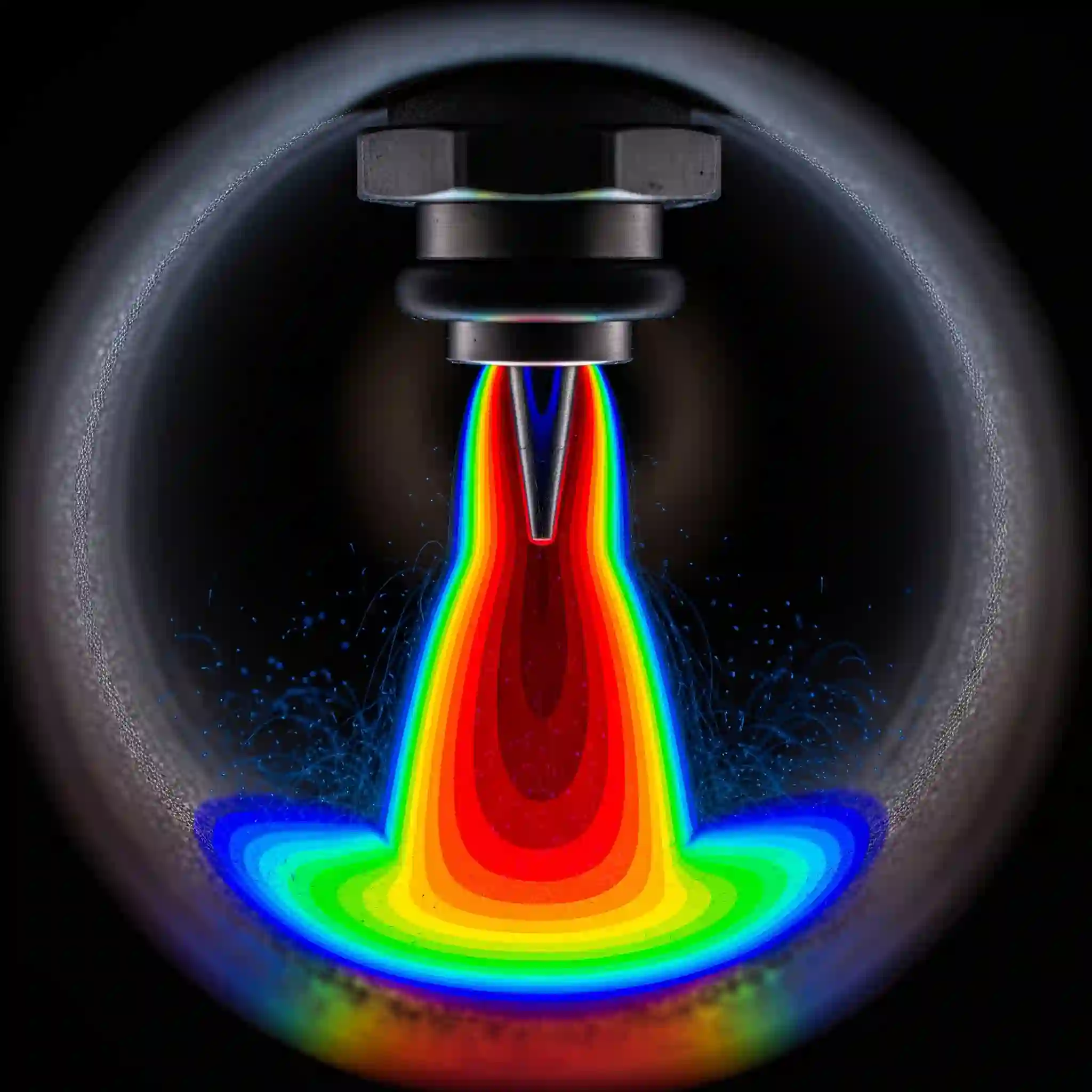
Shocks are the hallmark of supersonic flow. They aren’t smooth gradients; they’re near-instantaneous jumps in pressure, temperature, and density. To a numerical solver, this is a nightmare. It’s trying to solve a smooth equation across a physical cliff. 💥 If your mesh isn’t fine enough in the right places or your numerical scheme isn’t robust enough to handle the discontinuity, your solution will either smear the shock into a useless blur or, more likely, just diverge violently.
When Air Isn’t an Ideal Gas: The Importance of Real Gas Effects & Chemical Non-Equilibrium
Once you get into the hypersonic regime (typically Mach 5+), things get even wilder. The air heats up so much behind the shockwave that the molecules themselves start to vibrate and even break apart (dissociation). At this point, the ideal gas law is no longer valid. I remember working on a re-entry vehicle simulation where ignoring real gas effects led to a 30% under-prediction of the heat shield’s peak temperature. That’s the difference between a successful mission and a catastrophic failure. This is the kind of detail that separates academic exercises from industrial-grade analysis and is something expert CFD analysis companies look for when validating results.
The Challenge of Extreme Heat: Accurately Predicting Aerodynamic Heating and Thermal Loads
That intense heat has to go somewhere—right onto the surface of your vehicle. Predicting this aerodynamic heating is often the primary goal of the simulation. This isn’t just a thermal problem; its a structural one too. The massive thermal gradients can cause immense stress on the material. Accurately modeling this conjugate heat transfer (CHT) is crutial, and it often becomes the first step in understanding how these thermal loads interact with the structure in a more complex FSI analysis.
The Engineer’s Blueprint: Setting Up Your Supersonic Simulation for Success in Ansys Fluent/CFX
Alright, enough theory. Let’s get our hands dirty. How do we translate this physical understanding into a stable and accurate simulation setup? Your choice of solver and meshing strategy is everything.
Solver Selection: Why a Density-Based Solver is Non-Negotiable for Compressible Flows
This is the first and most important choice you’ll make. Most general-purpose CFD work uses a pressure-based solver. For high-speed flows, that’s a recipe for failure. You need a density-based solver. Why? Because it solves the continuity, momentum, and energy equations simultaneously (i.e., coupled). This tight coupling is essential for correctly capturing the physics where density changes dramatically.
Here’s a simple cheat sheet:
| Solver Type | Best For | Why it Works (or Fails) |
| Pressure-Based | Low-speed, incompressible/mildly compressible flows (Mach < 0.3) | Assumes pressure is the primary driver. Struggles when density changes are large and directly coupled to energy. |
| Density-Based | Transonic, supersonic, hypersonic flows (Mach > 0.3) | Solves for density as a primary variable. Built from the ground up to handle strong shocks and compressibility. |
Meshing Strategy That Works: From Shock Capturing with AMR to Resolving the Viscous Sublayer (y+ Control)
Your mesh has two main jobs: capture the shocks in the far-field and accurately resolve the incredibly thin boundary layer on the surface. For shocks, you need a high concentration of cells exactly where the shock forms. A fantastic tool for this is Adaptive Mesh Refinement (AMR), which automatically refines the mesh based on pressure gradients, saving you immense computational cost.
For the boundary layer, the y+ value is still king, but the rules change. Supersonic boundary layers are much thinner, so you need even more inflation layers packed tightly near the wall to get that desired y+ of ~1, especially if you want to predict heat transfer accurately. Skimping on the mesh here is a common mistake that leads to garbage results, no matter how good your solver settings are.
Turbulence Modeling in High-Speed Regimes: Choosing Between RANS (k-ω SST) and More Advanced Models
For turbulence, the good old k-ω SST model is often your best starting point. It’s robust and does a surprisingly good job handling the boundary layer separation that can occur behind shock interactions. But be aware of its limitations. In regions with massive separation or highly unsteady shocks, a RANS model will only give you a time-averaged approximation. It’s a reliable workhorse, but not a silver bullet.
Just as picking the right turbulence model is critical for capturing compressibility, choosing the right rheological model is essential when you’re dealing with different challenges, like simulating complex non-newtonian fluids in industrial mixers or pipelines. The core principle is the same: the model must match the physics.
“My Simulation Diverged!”: Troubleshooting Common Convergence Issues in High-Speed CFD
We’ve all seen it. The residual plot that looks like a seismograph during an earthquake before the solver finally gives up. 📉 Convergence is the biggest hurdle in high-speed CFD. Usually, the problem isn’t the software; it’s the setup. The solution is exploding because we’ve asked it to solve something that is physically or numerically impossible.
Nine times out of ten, the issue lies in one of the next two areas. I’ve spent countless late nights debugging simulations that failed because of a simple setting that seemed trivial at the time.
Taming Instability: Mastering the CFL Number, High-Order Schemes, and Solution Initialization
The Courant-Friedrichs-Lewy (CFL) number is your stability control knob. Think of it as a speed limit for how fast information can travel through your mesh in a single iteration. It’s temptng to crank it up to get faster results, but for high-speed flows, you must start low (e.g., CFL = 0.5 or even lower) and ramp it up gradually as the solution begins to stabilize.
Also, start your simulation with a first-order scheme to get a stable, albeit smeared, initial solution. Once the major flow features are established, you can switch to a hig-order scheme for accuracy. Rushing to a high-order scheme from the get-go on a poor initial guess is a classic way to make things go boom.
The Silent Killer: How Incorrect Boundary Conditions Can Ruin Your Results
This is the one that gets a lot of people. You can have the perfect mesh and solver settings, but a wrong boundary condition will poison the entire domain. A classic mistake is using a standard pressure-outlet on a boundary where a shock wave might exit. The boundary condition’s internal logic isn’t designed for supersonic flow, and it can cause the shock to unrealistically reflect back into your simulation, creating instabilities that kill convergence.
You need to use a far-field boundary condition designed for compressible flow. This same sensitivity to pressure settings is a huge factor in other domains, too—for example, it’s a primary cause of error when trying to predict cavitation in hydraulic machinery.
Beyond Colorful Contours: The CFDSource Framework for Validating Hypersonic Simulation Results
Getting a converged solution is only the beginning. How do you know if it’s right? Pretty pictures of shock diamonds are nice, but they don’t mean the drag prediction is accurate. Validation is what turns a CFD result from a colorful guess into an engineering tool. It’s a non-negotiable part of our process and a mark of any professional CFD services.
Benchmarking Against Reality: Using Wind Tunnel Data and Analytical Solutions for Validation
The gold standard is comparing your results to experimental data. There’s a wealth of public-domain wind tunnel data from NASA and other research institutions for classic shapes like cones, wedges, and cylinders at various Mach numbers. Compare your calculated shock angles, surface pressure coefficients (Cp), and heat transfer rates (Stanton number) against these trusted datasets. If your results match the experimental data, you can have confidence when you move on to your own unique design.
Case In Point: Simulating Re-entry Vehicle Aerothermodynamics – A CFDSource Project Snapshot
A few years back, we worked on a project to analyze the effectiveness of a control flap on a re-entry vehicle concept. The challenge was that at Mach 7, the shock wave from the vehicle’s nose would interact with the shock generated by the deflected flap. This “shock-shock interaction” created a tiny jet of extremely high pressure and heat right on the flap’s hinge. A simple simulation would miss this. By using AMR and a real gas model, we were able to capture this peak heating with precision, leading the design team to choose a more robust material for that specific location.
Your Next Step: From a Complex Simulation Challenge to an Actionable Engineering Solution
Hopefully, this gives you a clearer map for navigating the complexities of high-speed flow. It’s a field where details matter immensely, and experience often makes the difference between a failed run and a breakthrough insight.
Key Takeaways: A Pre-Run Checklist for Your Next High-Speed Flow Project
Before you hit “Calculate,” run through this quick list:
- Solver: Is it Density-Based?
- Gas Model: Is Ideal Gas valid, or do I need Real Gas effects?
- Mesh: Is it fine enough at the shock location and wall (y+ ~1)?
- CFL: Am I starting low and ramping up slowly?
- Schemes: Am I starting with 1st-order and switching to 2nd-order later?
- Boundaries: Am I using appropriate far-field conditions?
It’s a Demanding Field, But the Payoff is Huge
Mastering the challenges of simulating supersonic flow isn’t just an academic exercise; it’s a critical capability for modern aerospace design. From optimizing scramjets to ensuring the safety of re-entry vehicles, getting these simulations right pushes the boundaries of what’s possible. The process is demanding, but the engineering insights you gain are invaluable.