You’ve run the simulation. The solver converged, and you have a beautiful contour plot showing a temperature of precisely 450.5 K on a critical component. The job is done, right? Not quite.
For years, the number one question that keeps engineers up at night isn’t about convergence, it’s about confidence. How much can you really trust that single number? What if your inlet temperature fluctuates by just 2% in the real world, or the material properties aren’t exactly what the datasheet claims? This is where many standard CFD workflows fall short, and it’s a critical gap in many modern CFD simulation techniques. This guide is a practical introduction to Uncertainty Quantification (UQ). We’re going to move beyond that single, fragile number and into the world of robust, probabilistic design that gives you real confidence.
What is Uncertainty Quantification (UQ) and Why Should It Be Your Next Step in CFD?
Think of it this way. A standard CFD simulation is deterministic. You give it one set of inputs, you get one answer. UQ flips that on its head. It’s a probabilistic approach. You tell the simulation, “My inlet velocity isn’t exactly 10 m/s, it’s somewhere between 9.8 and 10.2 m/s.”
UQ then runs through the possibilities to tell you not just one outcome, but the range of possible outcomes and how likely each one is. It fundamentally changes your result from “The temperature is 85.3 °C” to “There is a 95% probability that the temperature will be between 82.1 °C and 88.5 °C.” That second statement is infinitely more valuable for making real-world engineering decisions.
From Deterministic to Probabilistic: The Core Shift in Engineering Mindset
This isn’t just a new tool; it’s a shift in thinking. For decades, we’ve relied on Safety Factors to account for the unknown. UQ is the analytical, data-driven version of that. It allows us to mathematically quantify our “gut feeling” about what might go wrong. Instead of over-engineering (and over-spending) with a large, arbitrary safety factor, you can make targeted design improvements based on what variables actually drive the uncertainty.
The High Cost of Ignoring Uncertainty: How “Small” Input Variations Can Lead to Major Design Failures
I’ll never forget a heat exchanger project from early in my career. Our simulation showed the design worked perfectly. But in deployment, it underperformed, narrowly avoiding a major failure. After weeks of investigation, we found the thermal conductivity of the supplied alloy varied by a tiny fraction from our simulation input. That ‘tiny’ difference was enough to throw everything off. The results was completely off. That was a scary lesson in how sensitive systems can be. Ignoring these small uncertainties isn’t just bad practice; it can be dangerous and incredibly expensive.
Identifying the “Unknowns”: Key Sources of Uncertainty in Your CFDSource Workflow
So where does this uncertainty come from? It’s everywhere, and learning to spot it is the first step. You have to put on your detective hat. 🤔 We generally group them into three main buckets. Honestly, just identifying these is a massive part of the battle, and it’s where a lot of the value in our CFD analysis services comes from—seeing the full picture. The process has become even more complex with the role of AI and PINNs in CFD, which introduces its own model uncertainties.
Parametric Uncertainty: Quantifying the Impact of Real-World Fluctuations (e.g., Inlet Conditions, Material Properties)
This is the most intuitive one. These are the numbers you type into your setup that have some variability in the real world:
- Boundary Conditions: Inlet flow rate, pressure, temperature. They are never perfectly steady.
- Material Properties: Viscosity, density, thermal conductivity, specific heat. These all can change with temperature or come with manufacturing tolerances.
- Geometric Tolerances: A manufactured pipe isn’t perfectly round. A surface isn’t perfectly smooth. These small geometric changes can matter.
Model Form Uncertainty: Is Your Turbulence Model (k-ε vs. k-ω SST) the Right Choice?
We’ve all been there, staring at the turbulence model dropdown in Fluent or CFX and wondering which one is “best.” Here’s the truth: all models are approximations of reality. The choice between k-epsilon, k-omega SST, or even a more advanced model like LES introduces uncertainty because each model makes different assumptions about the physics. Part of a robust analysis is understanding if your conclusions are overly dependent on that specific model choice.
Numerical Uncertainty: Acknowledging the Role of Mesh Resolutoin and Solver Settings
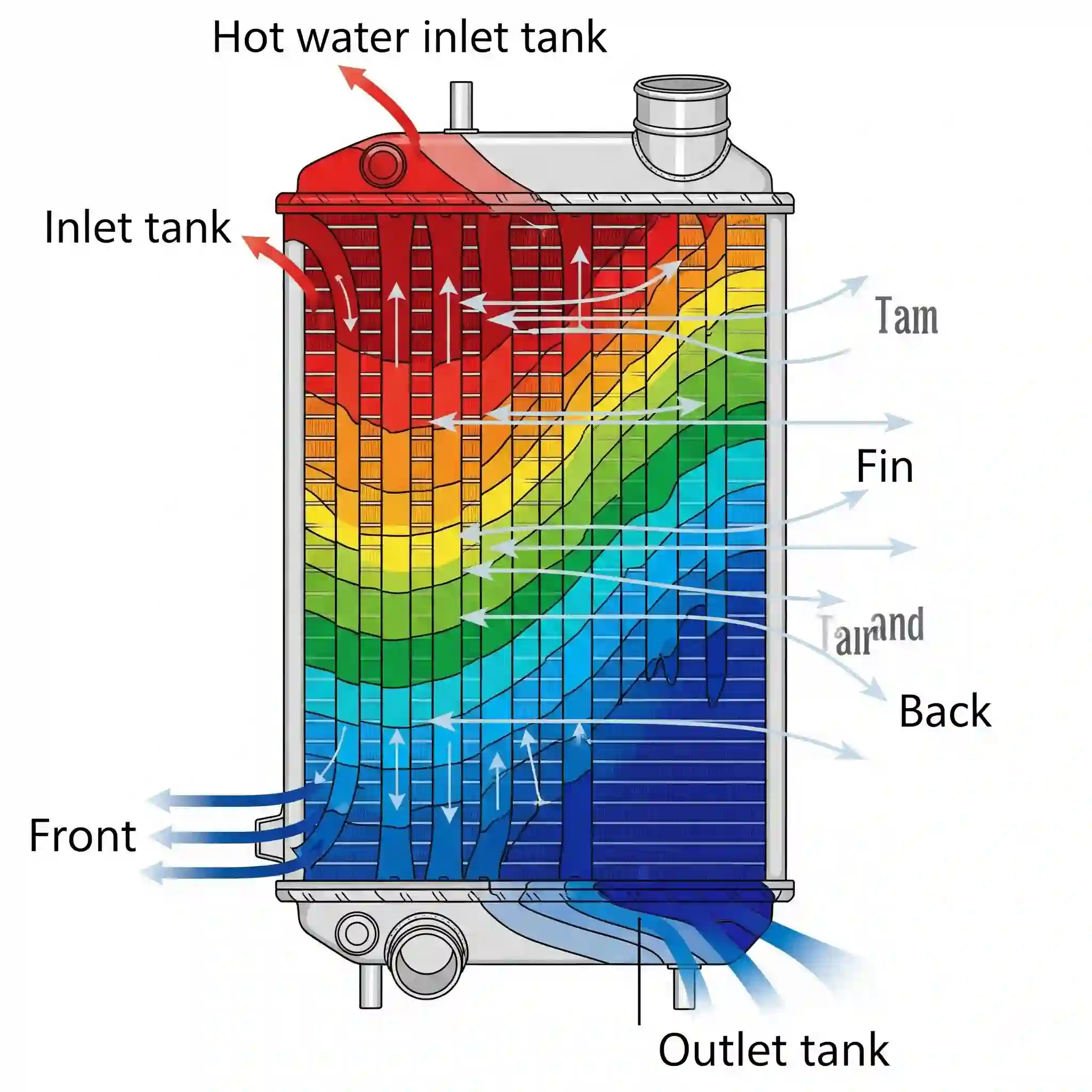
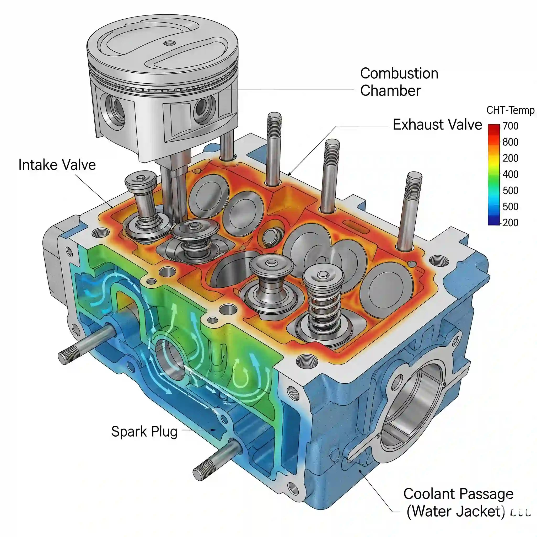
This type of uncertainty is introduced by us, the engineers, in the process of discretization. It’s the error that comes from the mesh not being infinitely fine or the convergence criteria not being infinitely strict. A coarse mesh might miss critical flow features, while an overly aggressive timestep in a transient simulation could smear out important physics. Running a proper mesh independence study is a basic form of quantifying this type of uncertainty, which becomes especially crucial when considering best practices for HPC in large simulations.
A Practical Overview of Common UQ Methods for Engineers
Alright, so we’ve identified our uncertainties. How do we actually process them? There are a bunch of methods, but for practical engineering, they usually boil down to two camps: the straightforward but slow way, and the smart but more complex way.
The “Brute Force” Method: When to Use Monte Carlo Simulations
Monte Carlo is the easiest to understand. Imagine you have three uncertain inputs. You randomly pick a value for each from their probability distributions, run one full CFD simulation, and record the result. Now, do that again. And again. Maybe 1,000 or 10,000 times. 🎲
This brute-force approach builds a statistically rich picture of your potential outcomes. The downside? It’s incredibly computationally expensive. If one simulation takes 8 hours, 1,000 of them is… well, you do the math. It’s often impractical unless you have serious access to high-performance computing clusters for your CFD work.
Smarter & Faster Approaches: An Introduction to Polynomial Chaos and Surrogate Models
This is where things get clever. Instead of running thousands of full simulations, these methods use a smaller, strategically chosen set of runs (maybe just 10-50) to build a mathematical approximation of your CFD model. This “surrogate model” or “response surface” is extremely fast to evaluate.
Once you have this fast approximation, you can run a million Monte Carlo iterations on it in seconds. It lets you explore the entire design space and calculate probabilities almost instantly. It’s more complex to set up initially, but the time savings are massive, especially for complex problems. These methods are the key to making Uncertainty Quantification (UQ) practical for industrial timelines.
Implementing UQ: A Step-by-Step Approach with Ansys and Other Commercial Solvers
Let’s get practical. How does this actually look in a tool like Ansys? Most major CFD packages now have built-in tools (like DesignXplorer in Ansys) to streamline this process. The workflow generally looks like this:
- Step 1: Defining Input Variables and Their Probability Distributions
This is the most critical step. You need to tell the software which parameters are uncertain and what their range of variation looks like. Is it a Normal distribution (a bell curve) around a mean value? Or is it a Uniform distribution (equally likely anywhere between a min and max)? This data comes from lab experiments, supplier datasheets, or even expert opinion. Garbage in, garbage out applies here more than anywhere else. - Step 2: Propagating Uncertainty Through Your CFD Model
Here, the UQ tool takes over. It acts as a “manager” for your CFD solver. It will automatically change the input parameters for each run according to the method you chose (e.g., Monte Carlo), launch the solver, wait for it to converge, and then scrape the key results you care about (like max temperature or pressure drop). - Step 3: Analyzing the Output: From Simple Contours to Rich Probabilistic Data
After all the runs are complete, you’re left with a mountain of information. This is no longer just one report file; it’s a dataset. The real challenge, and value, often lies in effectively handling and post-processing this large-scale data. The UQ tool will help you distill it into meaningful charts and statistics.
Interpreting UQ Results: What to Do with Your Newfound Knowledge
Having the results is one thing; using them to make better decisions is the whole point.
Sensitivity Analysis: Discovering Which Parameters Actually Drive Your Performance
This, for me, is the most powerful output of any UQ study. A sensitivity chart (often a tornado plot) shows you exactly how much each input uncertainty contributes to the output uncertainty. You might find that 80% of the variation in your component’s temperature is caused by the uncertainty in just one parameter: the inlet flow velocity. This tells you exactly where to focus your efforts. Don’t waste money tightening manufacturing tolerances on the part if the real problem is the unsteadiness of the pump feeding it!
Visualizing Confidence: Understanding Histograms, PDFs, and Confidence Intervals
Instead of a single value, you now get a histogram or a Probability Density Function (PDF) for your key outputs. This graph is your new best friend. It visually shows you the spread of possible outcomes. You can immediately see the most likely result (the peak of the curve) and, more importantly, the probability of hitting undesirable outcomes (the “tails” of the distribution). You can now confidently say, “There is less than a 1% chance of this part exceeding its critical temperature limit.” That’s a statement a project manager can truly work with.
The CFDSource Advantage: How We De-Risk Your Critical Projects Using UQ
We recently applied this to a project for an aerospace client developing a new winglet. Their deterministic CFD showed a 6% drag reduction. But they needed to know if that benefit would hold up across a range of real-world flight speeds and air densities.
Using a surrogate model-based UQ approach, we didn’t just confirm the drag reduction; we provided them with a probability map. It showed that in 95% of expected operational conditions, the drag reduction would be between 4.5% and 7.2%. It also highlighted that the winglet’s performance was most sensitive to the angle of attack at lower speeds. This insight allowed them to make a minor aerodynamic tweak that made the design far more robust, solidifying the business case and preventing a costly redesign later. This process is a foundational element for building a reliable digital twin of a physical asset, and its at the core of our CFD consulting services.
Putting It All Together: From Uncertainty to Engineering Insight
Moving from a single answer to a range of possibilities feels like a complication at first. But it’s not. It’s the path to clarity. It removes the guesswork and replaces it with calculated confidence. It transforms your CFD from a simple design tool into a powerful risk management asset. By embracing this mindset, you’re not just running a simulation; you’re truly understanding the behavior of your system. And that is the entire purpose of performing Uncertainty Quantification for more reliable CFD predictions.